Data Science with R is a new book by O'Reilly Media. Pre-order your copy at shop.oreilly.com.
Data Science with R is a new book by O'Reilly Media. Pre-order your copy at shop.oreilly.com.
“Tidy datasets are all alike but every messy dataset is messy in its own way.” – Hadley Wickham
Data science, at its heart, is a computer programming exercise. Data scientists use computers to store, transform, visualize, and model their data. As a result, every data science project begins with the same task: you must prepare your data to use it with a computer. In the wild, data sets come in many different formats, but each computer program expects your data to be organized in a predetermined way, which may vary from program to program.
In this book, we will use R to do data science. R is an excellent language for data science because with R you can do everything from collect your data (from the web or a database), to transform it, visualize it, explore it, model it, and run statistical tests on it. You can also use R to report your results when you are finished, and you can run R interactively, as if you were operating a calculator and not writing computer code. Best of all, R is free.
In this chapter, you will learn the best way to organize your data for R, a task that I call data tidying. This may seem like an odd place to start, but tidying data is the most fruitful skill you can learn as a data scientist. It will save you hours of time and make your data much easier to visualize, manipulate, and model with R.
Note that this chapter explains how to change the format, or layout, of tabular data. To learn how to use different file formats with R, see Appendix B: Data Sources.
In Section 2.1, you will learn how the features of R determine the best way to layout your data. This section introduces “tidy data,” a way to organize your data that works particularly well with R.
Section 2.2 teaches the basic method for making untidy data tidy. In
this section, you will learn how to reorganize the values in your data
set with the the spread() and gather() functions of the tidyr
package.
Section 2.3 explains how to split apart and combine values in your data set to make them easier to access with R.
Section 2.4 concludes the chapter, combining everything you’ve learned
about tidyr to tidy a real data set on tuberculosis epidemiology
collected by the World Health Organization.
You will need to have R installed on your computer to run the code in this chapter, as well as the RStudio IDE, a free program that makes it easier to use R. You can learn how to install both in Appendix A: Getting Started.
You will also need to install the tidyr, devtools, and DSR
packages. To install, tidyr and devtools, open RStudio and run the
command
install.packages(c("tidyr", "devtools"))
DSR is a collection of data sets that I have assembled for this book
and saved online as a github repository
(github.com/garrettgman/DSR). To
install DSR, run the command
devtools::install_github("garrettgman/DSR")
You can organize tabular data in many ways. For example, the data sets
below show the same data organized in four different ways. Each data set
shows the same values of four variables country, year, population,
and cases, but each data set organizes the values into a different
layout . You can access the data sets in the DSR package.
library(DSR)

# Data set one
table1

## Source: local data frame [6 x 4]
##
##       country year  cases population
## 1 Afghanistan 1999    745   19987071
## 2 Afghanistan 2000   2666   20595360
## 3      Brazil 1999  37737  172006362
## 4      Brazil 2000  80488  174504898
## 5       China 1999 212258 1272915272
## 6       China 2000 213766 1280428583

# Data set two
table2

## Source: local data frame [12 x 4]
##
##        country year        key      value
## 1  Afghanistan 1999      cases        745
## 2  Afghanistan 1999 population   19987071
## 3  Afghanistan 2000      cases       2666
## 4  Afghanistan 2000 population   20595360
## 5       Brazil 1999      cases      37737
## 6       Brazil 1999 population  172006362
## 7       Brazil 2000      cases      80488
## 8       Brazil 2000 population  174504898
## 9        China 1999      cases     212258
## 10       China 1999 population 1272915272
## 11       China 2000      cases     213766
## 12       China 2000 population 1280428583

# Data set three
table3

## Source: local data frame [6 x 3]
##
##       country year              rate
## 1 Afghanistan 1999      745/19987071
## 2 Afghanistan 2000     2666/20595360
## 3      Brazil 1999   37737/172006362
## 4      Brazil 2000   80488/174504898
## 5       China 1999 212258/1272915272
## 6       China 2000 213766/1280428583
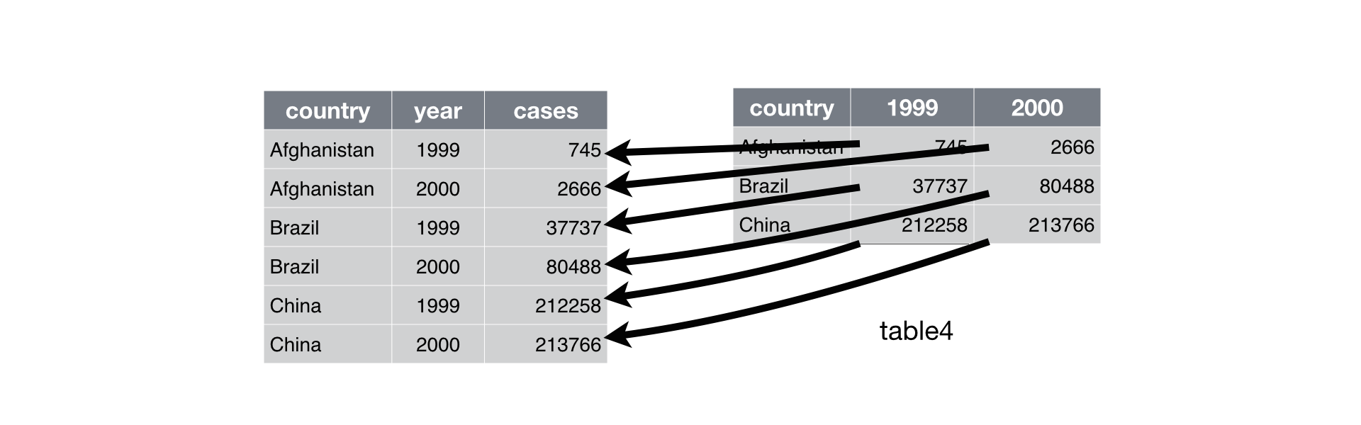
The last data set is a collection of two tables.
# Data set four
table4  # cases

## Source: local data frame [3 x 3]
##
##       country   1999   2000
## 1 Afghanistan    745   2666
## 2      Brazil  37737  80488
## 3       China 212258 213766

table5  # population

## Source: local data frame [3 x 3]
##
##       country       1999       2000
## 1 Afghanistan   19987071   20595360
## 2      Brazil  172006362  174504898
## 3       China 1272915272 1280428583
You might think that these data sets are interchangeable since they display the same information, but one data set will be much easier to work with in R than the others.
Why should that be?
R follows a set of conventions that makes one layout of tabular data much easier to work with than others. Your data will be easier to work with in R if it follows three rules
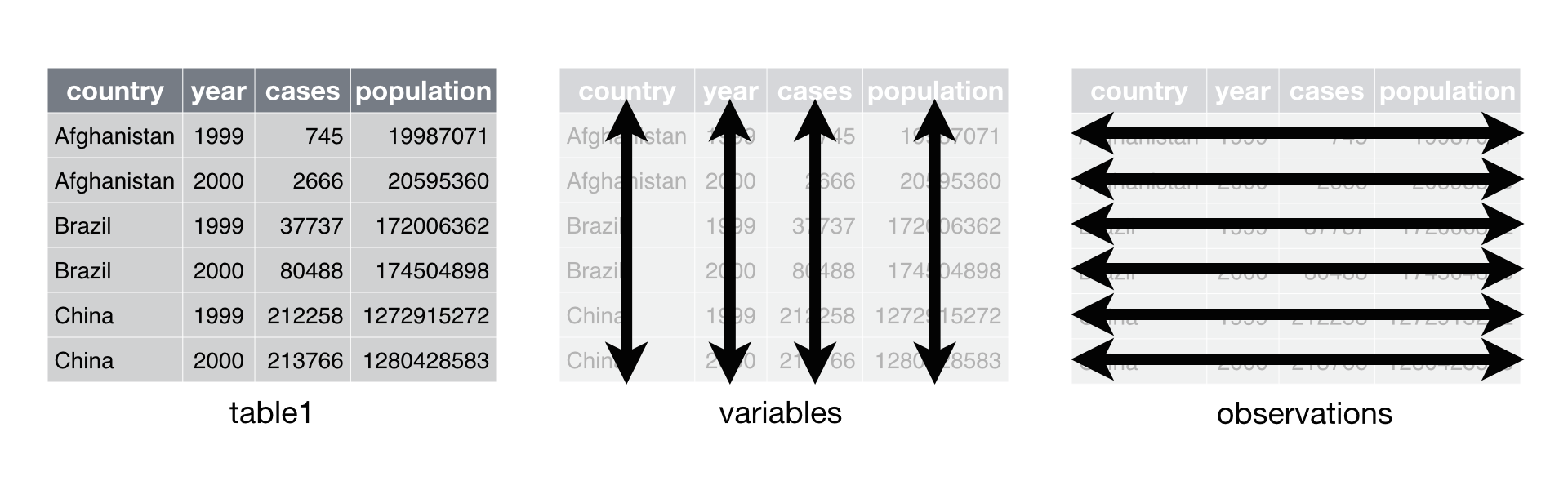
Data that satisfies these rules is known as tidy data. Notice that
table1 is tidy data.
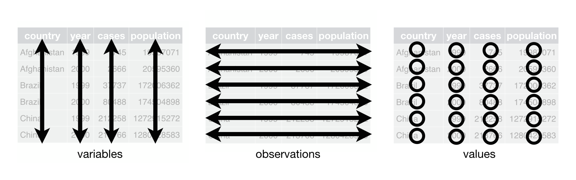 In
In table1, each variable is
placed in its own column, each observation in its own row, and each
value in its own cell.
Tidy data builds on a premise of data science that data sets contain both values and relationships. Tidy data displays the relationships in a data set as consistently as it displays the values in a data set.
At this point, you might think that tidy data is so obvious that it is trivial. Surely, most data sets come in a tidy format, right? Wrong. In practice, raw data is rarely tidy and is much harder to work with as a result. Section 2.4 provides a realistic example of data collected in the wild.
Tidy data works well with R because R is a vectorized programming language. Data structures in R are built from vectors and R’s operations are optimized to work with vectors. Tidy data takes advantage of both of these traits.
R stores tabular data as a data frame, a list of atomic vectors arranged to look like a table. Each column in the table is an atomic vector in the list.
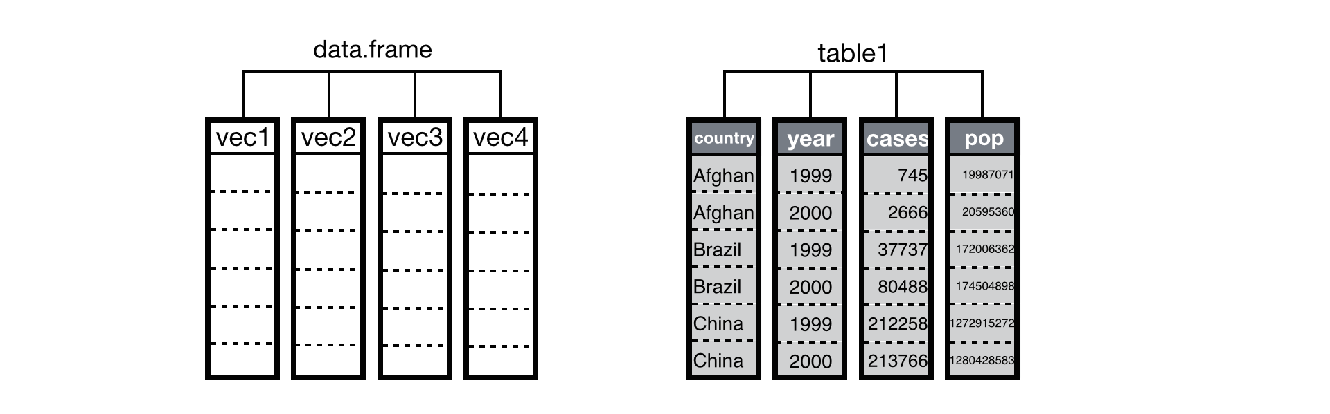 A data frame is a
list of vectors that R displays as a table. When your data is tidy, the
values of each variable fall in their own column vector.
A data frame is a
list of vectors that R displays as a table. When your data is tidy, the
values of each variable fall in their own column vector.
Tidy data arranges values so that the relationships in the data parallel the structure of the data frame. Recall that each data set is a collection of values associated with a variable and an observation. In tidy data, each variable is assigned to its own column, i.e., its own vector in the data frame. As a result, you can extract easily the values of a variable in a tidy data set with R’s list syntax,
table1$cases

## [1]    745   2666  37737  80488 212258 213766
R will return the values as an atomic vector, one of the most versatile data structures in R. Many functions in R are written to take atomic vectors as input, as are R’s mathematical operators. This adds up to an easy user experience; you can extract and manipulate the values of variables in tidy data with concise, simple code, e.g.,
mean(table1$cases)

## [1] 91276.67

table1$cases / table1$population * 10000

## [1] 0.372741 1.294466 2.193930 4.612363 1.667495 1.669488
Tidy data also takes advantage of R’s vectorized operations. In R, it is common to supply one or more vectors of values to a function or mathematical operator as input, and to receive a vector of values as output. To create the output, R applies the function in element-wise fashion: R first applies the function (or operation) to the first elements of each vector involved. Then R applies the function (or operation) to the second elements of each vector involved, and so on until R reaches the end of the vectors. If one vector is shorter than the others, R will recycle its values as needed (according to a set of recycling rules).

If your data is tidy, element-wise execution will ensure that observations are preserved across functions and operations. Each value will only be paired with other values that appear in the same row of the data frame.
Do these small advantages matter in the long run? Yes. Consider what it would be like to do a simple calculation with each of the data sets from the start of the section.
Assume that in these data sets, cases refers to the number of people
diagnosed with TB per country per year. To calculate the rate of TB
cases per country per year (i.e, the number of people per 10,000
diagnosed with TB), you will need to do four operations with the data.
You will need to:
If you use basic R syntax, your calculations will look like the code below. If you’d like to brush up on basic R syntax, see Appendix A: Getting Started.
Since table1 is organized in a tidy fashion, you can calculate the
rate like this,
# Data set one
table1$cases / table1$population * 10000
Data set two intermingles the values of population and cases in the same columns. As a result, you will need to untangle the values whenever you want to work with each variable separately.
You’ll need to perform an extra step to calculate the rate.
# Data set two
case_rows <- c(1, 3, 5, 7, 9, 11, 13, 15, 17)
pop_rows <- c(2, 4, 6, 8, 10, 12, 14, 16, 18)
table2$value[case_rows] / table2$value[pop_rows] * 10000
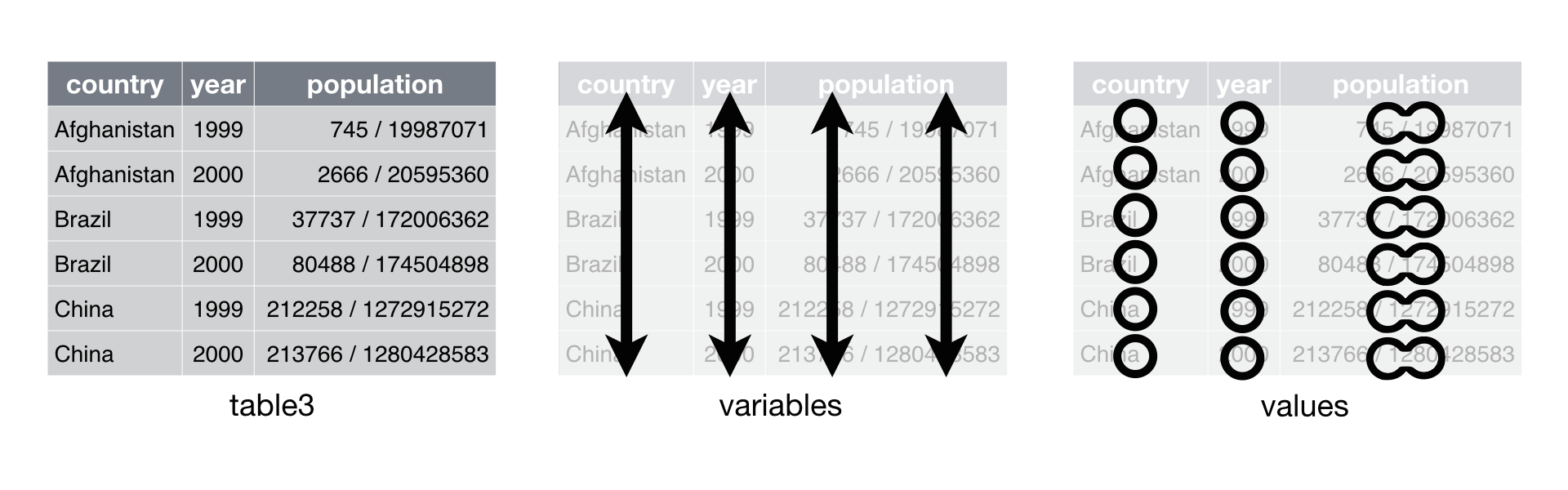
Data set three combines the values of cases and population into the same cells. It may seem that this would help you calculate the rate, but that is not so. You will need to separate the population values from the cases values if you wish to do math with them. This can be done, but not with “basic” R syntax.
# Data set three
# No basic solution
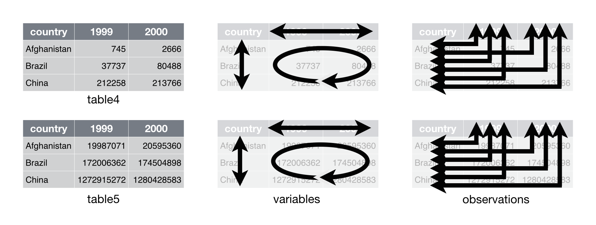
Data set four stores each variable in a different format: as a column, a
set of column names, or a field of cells. As a result, you will need to
work with each variable differently. This makes code written for data
set four hard to generalize. The code that extracts the values of
year, names(table4)[-1], cannot be generalized to extract the values
of population, c(table5$1999, table5$2000, table5$2001). Compare this
to data set one. With table1, you can use the same code to extract the
values of year, table1$year, that you use to extract the values of
population. To do so, you only need to change the name of the variable
that you will access: table1$population.
The organization of data set four is inefficient in a second way as well. Data set four separates the values of some variables across two separate tables. This is inconvenient because you will need to extract information from two different places whenever you want to work with the data.
After you collect your input, you can calculate the rate.
# Data set four
cases <- c(table4$1999, table4$2000, table4$2001)
population <- c(table5$1999, table5$2000, table5$2001)
cases / population * 10000
Data set one is much easier to work with than with data sets two, three, or four. To work with data sets two, three, and four, you need to take extra steps, which makes your code harder to write, harder to understand, and harder to debug.
Keep in mind that this is a trivial calculation with a trivial data set. The energy you must expend to manage a poor layout will increase with the size of your data. Extra steps will accumulate over the course of an analysis and allow errors to creep into your work. You can avoid these difficulties by converting your data into a tidy format at the start of your analysis.
The next sections will show you how to transform untidy data sets into tidy data sets.
Tidy data was popularized by Hadley Wickham, and it serves as the basis for many R packages and functions. You can learn more about tidy data by reading Tidy Data a paper written by Hadley Wickham and published in the Journal of Statistical Software. Tidy Data is available online at www.jstatsoft.org/v59/i10/paper.
spread() and gather()The tidyr package by Hadley Wickham is designed to help you tidy your
data. It contains four functions that alter the layout of tabular data
sets, while preserving the values and relationships contained in the
data sets.
The two most important functions in tidyr are gather() and
spread(). Each relies on the idea of a key value pair.
A key value pair is a simple way to record information. A pair contains two parts: a key that explains what the information describes, and a value that contains the actual information. So for example,
Password: 0123456789
would be a key value pair. 0123456789 is the value, and it is
associated with the key Password.
Data values form natural key value pairs. The value is the value of the
pair and the variable that the value describes is the key. So for
example, you could decompose table1 into a group of key value pairs,
but it would cease to be a useful data set because you no longer know
which values belong to the same observation.
Country: Afghanistan
Country: Brazil
Country: China
Year: 1999
Year: 2000
Year: 2001
Population:   19987071
Population:   20595360
Population:  172006362
Population:  174504898
Population: 1272915272
Population: 1280428583
Cases:    745
Cases:   2666
Cases:  37737
Cases:  80488
Cases: 212258
Cases: 213766
Every cell in a table of data contains one half of a key value pair, as
does every column name. In tidy data, each cell will contain a value and
each column name will contain a key, but this doesn’t need to be the
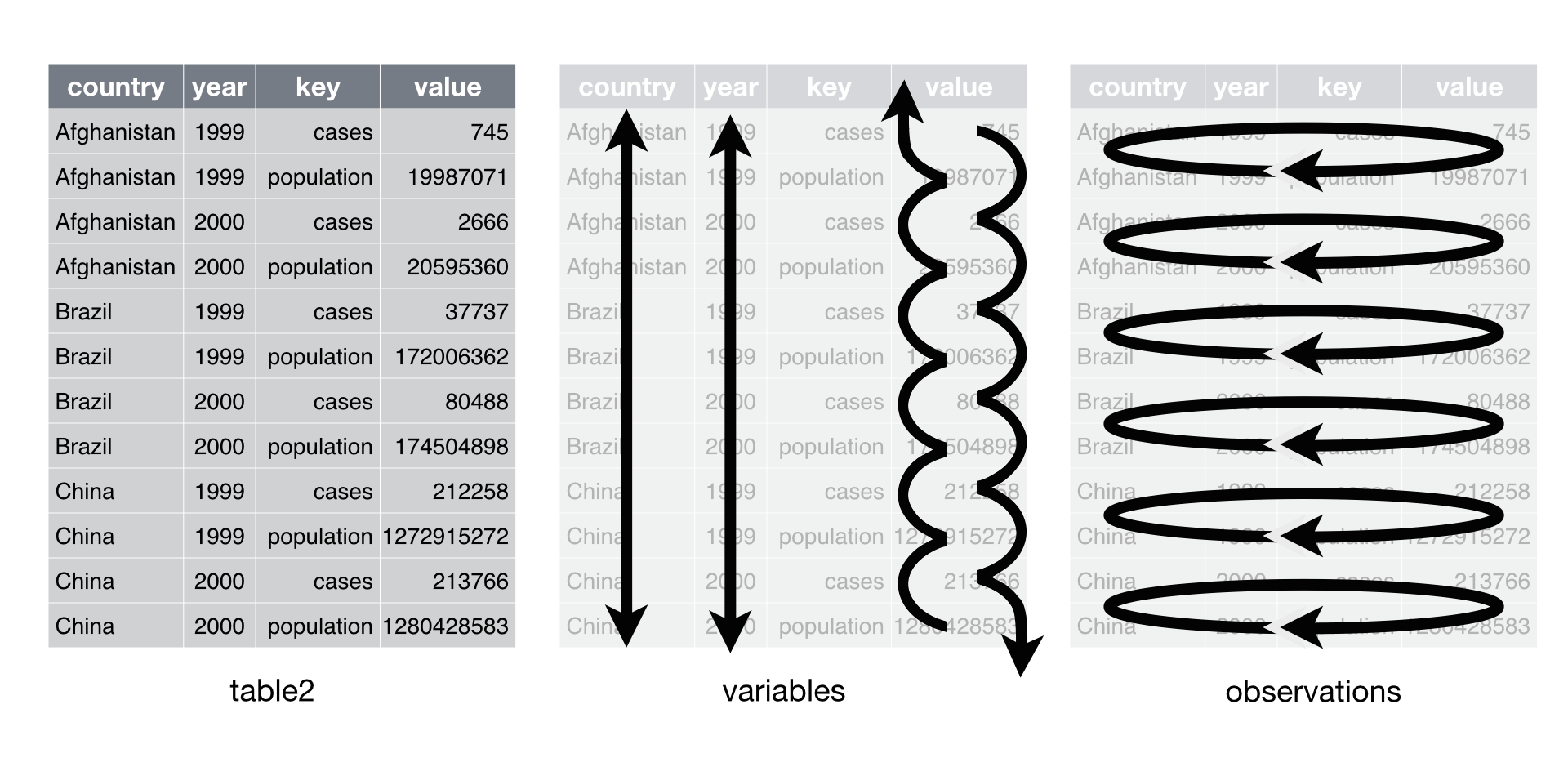
case for untidy data. Consider table2.
table2

## Source: local data frame [12 x 4]
##
##        country year        key      value
## 1  Afghanistan 1999      cases        745
## 2  Afghanistan 1999 population   19987071
## 3  Afghanistan 2000      cases       2666
## 4  Afghanistan 2000 population   20595360
## 5       Brazil 1999      cases      37737
## 6       Brazil 1999 population  172006362
## 7       Brazil 2000      cases      80488
## 8       Brazil 2000 population  174504898
## 9        China 1999      cases     212258
## 10       China 1999 population 1272915272
## 11       China 2000      cases     213766
## 12       China 2000 population 1280428583
In table2, the key column contains only keys (and not just because
the column is labelled key). Conveniently, the value column contains
the values associated with those keys.
You can use the spread() function to tidy this layout.
spread()spread() turns a pair of key:value columns into a set of tidy columns.
To use spread(), pass it the name of a data frame, then the name of
the key column in the data frame, and then the name of the value column.
Pass the column names as they are; do not use quotes.
To tidy table2, you would pass spread() the key column and then
the value column.
table2

## Source: local data frame [12 x 4]
##
##        country year        key      value
## 1  Afghanistan 1999      cases        745
## 2  Afghanistan 1999 population   19987071
## 3  Afghanistan 2000      cases       2666
## 4  Afghanistan 2000 population   20595360
## 5       Brazil 1999      cases      37737
## 6       Brazil 1999 population  172006362
## 7       Brazil 2000      cases      80488
## 8       Brazil 2000 population  174504898
## 9        China 1999      cases     212258
## 10       China 1999 population 1272915272
## 11       China 2000      cases     213766
## 12       China 2000 population 1280428583

library(tidyr)
spread(table2, key, value)

## Source: local data frame [6 x 4]
##
##       country year  cases population
## 1 Afghanistan 1999    745   19987071
## 2 Afghanistan 2000   2666   20595360
## 3      Brazil 1999  37737  172006362
## 4      Brazil 2000  80488  174504898
## 5       China 1999 212258 1272915272
## 6       China 2000 213766 1280428583
spread() returns a copy of your data set that has had the key and
value columns removed. In their place, spread() adds a new column for
each unique value of the key column. These unique values will form the
column names of the new columns. spread() distributes the cells of the
former value column across the cells of the new columns and truncates
any non-key, non-value columns in a way that prevents duplication.
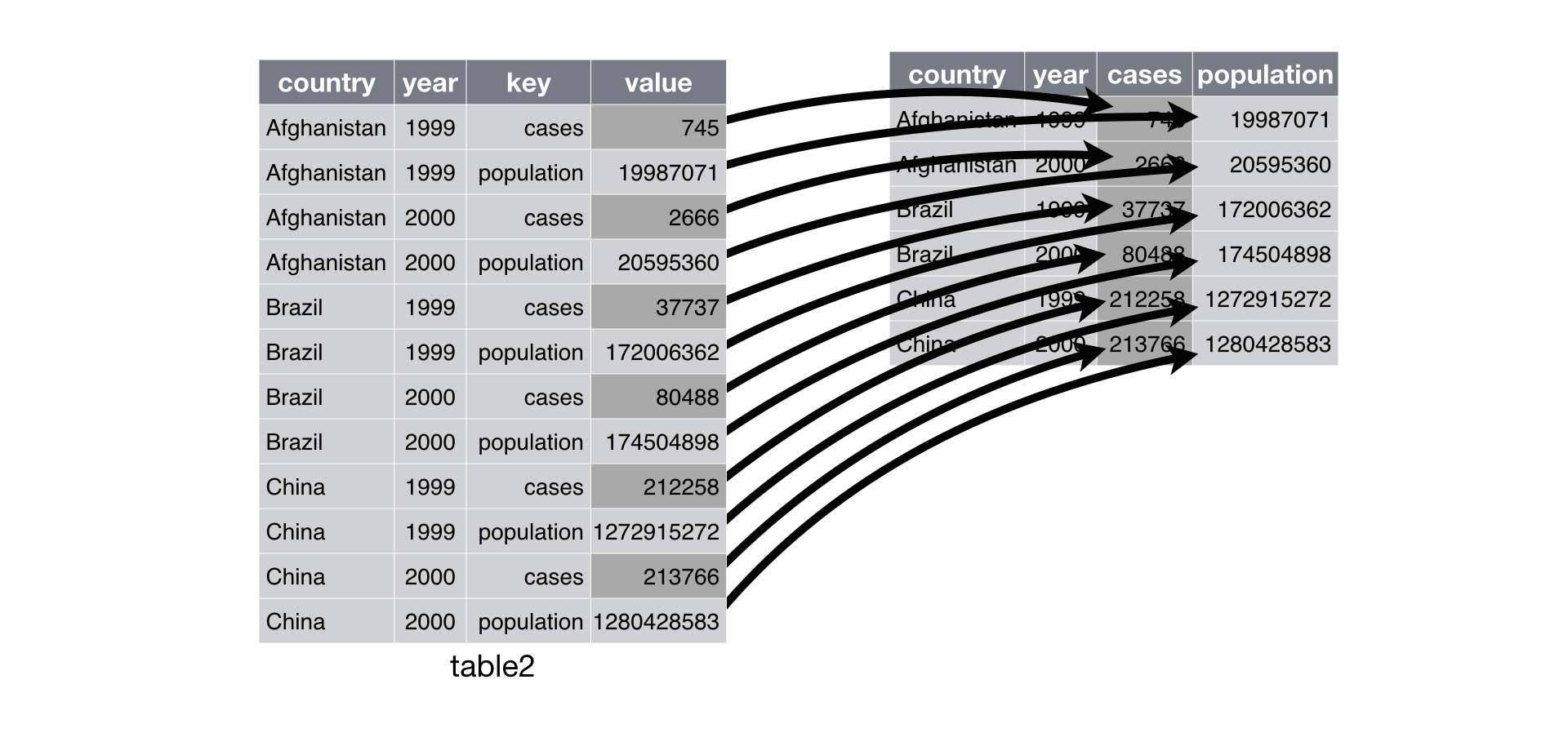
spread() distributes a pair of
key:value columns into a field of cells. The unique values of the key
column become the column names of the field of cells.
You can see that spread() maintains each of the relationships
expressed in the original data set. The output contains the four
original variables, country, year, population, and cases.
And the values of these variables are grouped according to the orginal observations, but now the layout of these relationships is tidy.
spread() takes three optional arguments in addition to data, key,
and value:
fill - If the tidy structure creates combinations of variables
that do not exist in the original data set, spread() will place an
NA in the resulting cells. NA is R’s missing value symbol. You
can change this behaviour by passing fill an alternative value to
use.
convert - If a value column contains multiple types of data,
its elements will be saved as a single type, usually character
strings. As a result, the new columns created by spread() will
also contain character strings. If you set convert = TRUE,
spread() will run type.convert() on each new column, which will
convert strings to doubles (numerics), integers, logicals,
complexes, or factors.
drop - The drop argument controls how spread() handles
factors in the key column. If you set drop = FALSE, spread will
keep factor levels that do not appear in the key column, filling in
the missing combinations with the value of fill.
gather()gather() does the reverse of spread(). gather() collects a set of
column names and places them into a single “key” column. It also
collects the cells of those columns and places them into a single value
column. You can use gather() to tidy table4.
table4  # cases

## Source: local data frame [3 x 3]
##
##       country   1999   2000
## 1 Afghanistan    745   2666
## 2      Brazil  37737  80488
## 3       China 212258 213766
To use gather(), pass it the name of a data frame to reshape. Then
pass gather() a character string to use for the name of the “key”
column that it will make, as well as a character string to use as the
name of the value column that it will make. Finally, specify which
columns gather() should collapse into the key value pair (here with
integer notation).
gather(table4, "year", "cases", 2:3)

## Source: local data frame [6 x 3]
##
##       country year  cases
## 1 Afghanistan 1999    745
## 2      Brazil 1999  37737
## 3       China 1999 212258
## 4 Afghanistan 2000   2666
## 5      Brazil 2000  80488
## 6       China 2000 213766
gather() returns a copy of the data frame with the specified columns
removed. To this data frame, gather() has added two new columns: a
“key” column that contains the former column names of the removed
columns, and a value column that contains the former values of the
removed columns. gather() repeats each of the former column names (as
well as each of the original columns) to maintain each combination of
values that appeared in the original data set. gather() uses the first
string that you supplied as the name of the new “key” column, and it
uses the second string as the name of the new value column.
I’ve placed “key” in quotation marks because you will usually use
gather() to create tidy data. In this case, the “key” column will
contain values, not keys. The values will only be keys in the sense that
they were formally in the column names, a place where keys belong.
Just like spread(), gather maintains each of the relationships in the
original data set. This time table3 only contained three variables,
country, year and cases. Each of these appears in the output of
gather() in a tidy fashion.
gather() also maintains each of the observations in the original data
set, organizing them in a tidy fashion.
We can use gather() to tidy table4 in a similar fashion.
table5  # population

## Source: local data frame [3 x 3]
##
##       country       1999       2000
## 1 Afghanistan   19987071   20595360
## 2      Brazil  172006362  174504898
## 3       China 1272915272 1280428583

gather(table5, "year", "population", 2:3)

## Source: local data frame [6 x 3]
##
##       country year population
## 1 Afghanistan 1999   19987071
## 2      Brazil 1999  172006362
## 3       China 1999 1272915272
## 4 Afghanistan 2000   20595360
## 5      Brazil 2000  174504898
## 6       China 2000 1280428583
In this code, I identified the columns to collapse with a series of
integers. 2:3 describes the second and third columns of the data
frame. You can identify the same columns with each of the commands
below.
gather(table5, "year", "population", c(2, 3))
gather(table5, "year", "population", -1)
You can also identify columns by name with the notation introduced by
the select function in dplyr, see Section 3.1.
In Section 3.6, you will learn how to combine two data frames, like
the tidy versions of table4 and table5 into a single data frame.
separate() and unite()spread() and gather() help you reshape the layout of your data to
place variables in columns and observations in rows. separate() and
unite() help you split and combine cells to place a single, complete
value in each cell.
separate()separate() turns a single character column into multiple columns by
splitting the values of the column wherever a separator character
appears.
[SEPARATE DIAGRAM] ![]()
So, for example, we can use separate() to tidy table3, which
combines values of cases and population in the same column.
separate(table3, rate, into = c("cases", "population"))

## Source: local data frame [6 x 4]
##
##       country year  cases population
## 1 Afghanistan 1999    745   19987071
## 2 Afghanistan 2000   2666   20595360
## 3      Brazil 1999  37737  172006362
## 4      Brazil 2000  80488  174504898
## 5       China 1999 212258 1272915272
## 6       China 2000 213766 1280428583
To use separate() pass separate the name of a data frame to reshape
and the name of a column to separate. Also give separate() an into
argument, which should be a vector of character strings to use as new
column names. separate() will return a copy of the data frame with the
column removed. The previous values of the column will be split across
several columns, one for each name in into.
By default, separate() will split values wherever a non-alphanumeric
character appears. Non-alphanumeric characters are characters that are
neither a number nor a letter. For example, in the code above,
separate() split the values of rate at the forward slash characters.
If you wish to use a specific character to separate a column, you can
pass the character to the sep argument of separate(). For example,
we could rewrite the code above as
separate(table3, rate, into = c("cases", "population"), sep = "/")
See Appendix E to learn more about regular expressions in R.
You can also pass an integer or vector of integers to sep.
separate() will interpret the integers as positions to split at.
Positive values start at 1 at the far-left of the strings; negative
value start at -1 at the far-right of the strings. The length of sep
should be one less than the number of names in into. You can use this
arrangement to separate the last two digits of each year.
separate(table3, year, into = c("century", "year"), sep = 2)

## Source: local data frame [6 x 4]
##
##       country century year              rate
## 1 Afghanistan      19   99      745/19987071
## 2 Afghanistan      20   00     2666/20595360
## 3      Brazil      19   99   37737/172006362
## 4      Brazil      20   00   80488/174504898
## 5       China      19   99 212258/1272915272
## 6       China      20   00 213766/1280428583
You can futher customize separate() with the remove, convert, and
extra arguments:
remove - Set remove = FALSE to retain the column of values
that were separated in the final data frame.convert - By default, separate() will return new columns as
character columns. Set convert = TRUE to convert new columns to
double (numeric), integer, logical, complex, and factor columns with
type.convert().extra - extra controls what happens when the number of new
values in a cell does not match the number of new columns in into.
If extra = error (the default), separate() to return an error.
If extra = drop, separate() will drop new values and supply
NAs as necessary to fill the new columns. If extra = merge,
separate() will split at most length(into) times.unite()unite() does the opposite of separate(): it combines multiple
columns into a single column.
[UNITE DESCRIPTION] ![]()
We can use unite() to rejoin the century and year columns that we
created in the last example. That data is saved in the DSR package as
table6.
table6

## Source: local data frame [6 x 4]
##
##       country century year              rate
## 1 Afghanistan      19   99      745/19987071
## 2 Afghanistan      20   00     2666/20595360
## 3      Brazil      19   99   37737/172006362
## 4      Brazil      20   00   80488/174504898
## 5       China      19   99 212258/1272915272
## 6       China      20   00 213766/1280428583

unite(table6, "new", century, year, sep = "")

## Source: local data frame [6 x 3]
##
##       country  new              rate
## 1 Afghanistan 1999      745/19987071
## 2 Afghanistan 2000     2666/20595360
## 3      Brazil 1999   37737/172006362
## 4      Brazil 2000   80488/174504898
## 5       China 1999 212258/1272915272
## 6       China 2000 213766/1280428583
Give unite() the name of the data frame to reshape, the name of the
new column to create (as a character string), and the names of the
columns to unite. unite() will place an underscore (_) between values
from separate columns. If you would like to use a different separator,
or no separator at all, pass the separator as a character string to
sep.
unite() returns a copy of the data frame that includes the new column,
but not the columns used to build the new column. If you would like to
retain these columns, add the argument remove = FALSE.
You can also use integers or the syntax of the dplyr::select to
specify columns to unite in a more concise way. We’ll learn about
select in Section 3.1.
The who data set in the DSR package contains cases of tuberculosis
(TB) reported between 1995 and 2013 sorted by country, age, and gender.
The data comes in the 2014 World Health Organization Global
Tuberculosis Report, available for download at
www.who.int/tb/country/data/download/en/.
The data provides a wealth of epidemiological information, but it would
be difficult to work with the data as it is.
To see the data in its raw form, load DSR with library(DSR) then run
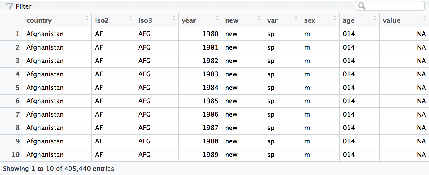
View(who)
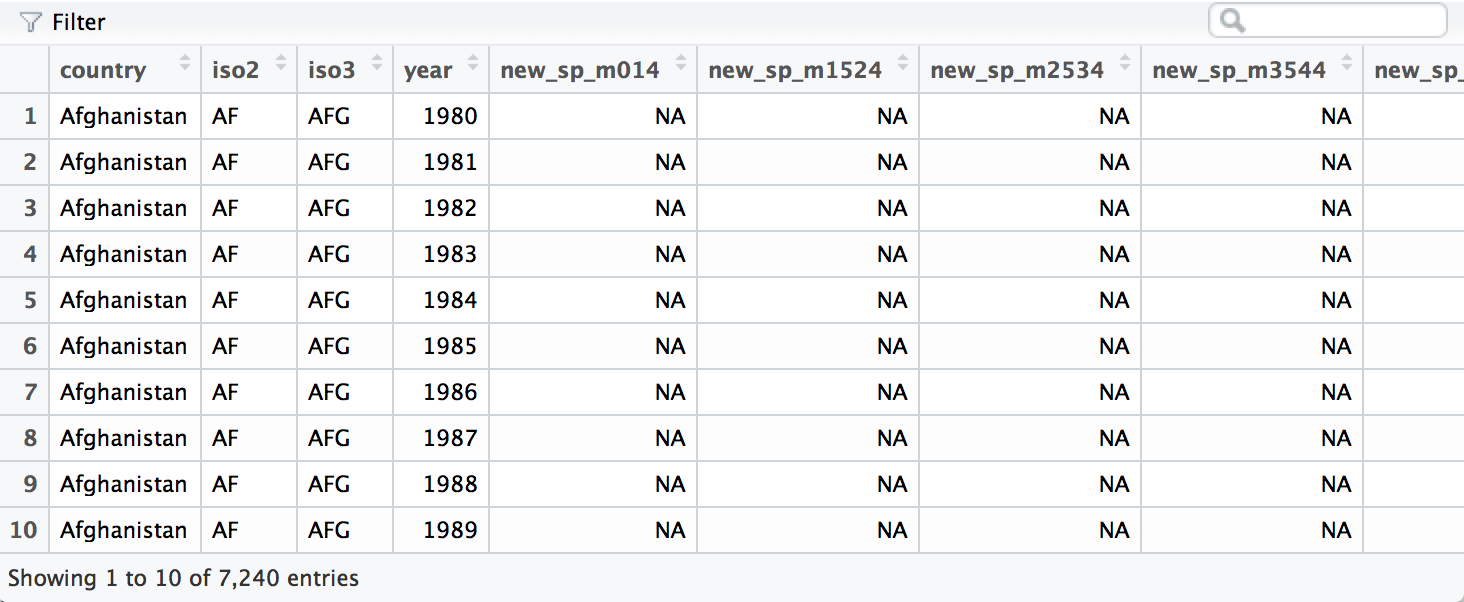
A subset of the who data frame displayed with
View().
who provides a realistic example of tabular data in the wild. It
contains redundant columns, odd variable codes, and many missing values.
In short, who is messy.
TIP
The View() function opens a data viewer in the RStudio IDE. Here you
can examine the data set, search for values, and filter the display
based on logical conditions. Notice that the View() function begins
with a capital V.
The most unique feature of who is its coding system. Columns five
through sixty encode four separate pieces of information in their column
names:
The first three letters of each column denote whether the column contains new or old cases of TB. In this data set, each column contains new cases.
rel stands for cases of relapseep stands for cases of extrapulmonary TBsn stands for cases of pulmonary TB that could not be
diagnosed by a pulmonary smear (smear negative)sp stands for cases of pulmonary TB that could be diagnosed be
a pulmonary smear (smear positive)The sixth letter describes the sex of TB patients. The data set
groups cases by males (m) and females (f).
014 stands for patients that are 0 to 14 years old1524 stands for patients that are 15 to 24 years old2534 stands for patients that are 25 to 34 years old3544 stands for patients that are 35 to 44 years old4554 stands for patients that are 45 to 54 years old5564 stands for patients that are 55 to 64 years old65 stands for patients that are 65 years old or olderNotice that the who data set is untidy in multiple ways. First, the
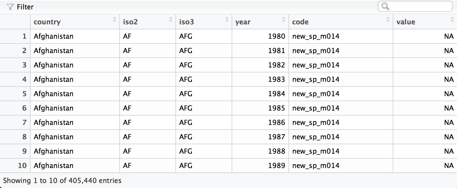
data appears to contain values in its column names. We can move the
values into their own column with gather(). This will make it easy to
separate the values combined in each code.
who <- gather(who, "code", "value", 5:60)
We can separate the values in each code with two passes of separate().
The first pass will split the codes at each underscore.
who <- separate(who, code, c("new", "var", "sexage"))
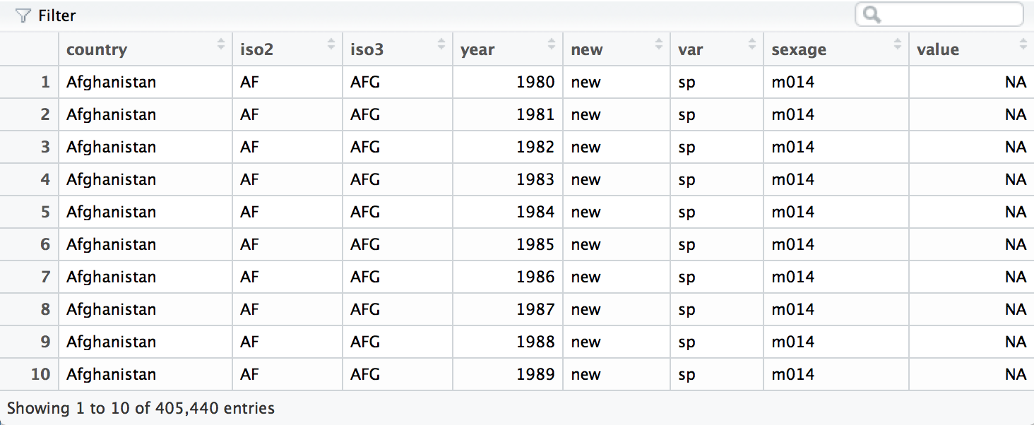
The second pass will split sexage after the first character to create
a sex column and an age column.
who <- separate(who, sexage, c("sex", "age"), sep = 1)
Finally, we can move the rel, ep, sn, and sp keys into their own
column names with spread().
who <- spread(who, var, value)
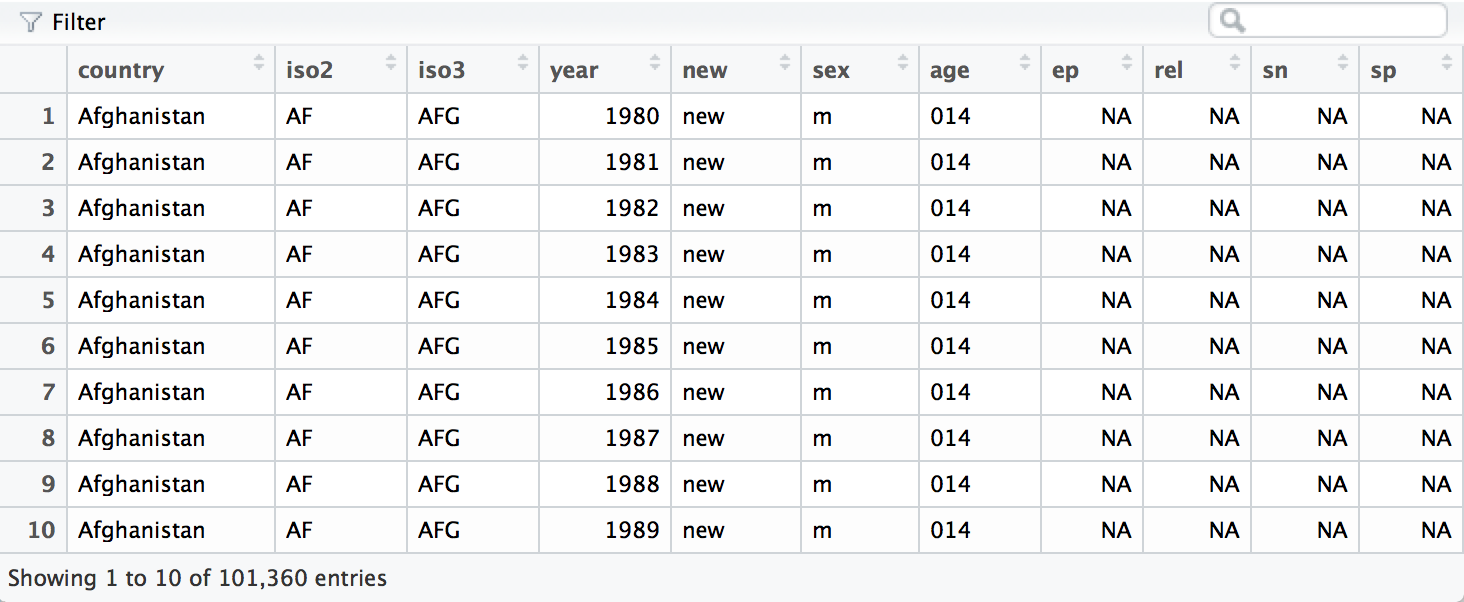
The who data set is now tidy. It is far from sparkling (for example,
it contains several redundant columns), but it will now be much easier
to work with in R. We will continue to work with this tidy version of
who in Section 3.7, where we will remove the redundant columns and
calculate new variables.