Creating Shiny Widgets

The shinyApp Function

At their core Shiny widgets are mini-applications created using the shinyApp function. Rather than create a ui.R and server.R as you would for a typical Shiny application, you pass the ui and server definitions to the shinyApp function as arguments. For example:

shinyApp(
  ui = fluidPage(
    selectInput("region", "Region:", choices = colnames(WorldPhones)),
    plotOutput("phonePlot")
  ),
  server = function(input, output) {
    output$phonePlot <- renderPlot({
      barplot(WorldPhones[,input$region]*1000, 
              ylab = "Number of Telephones", xlab = "Year")
    })
  },
  options = list(height = 500)
)

The simplest type of Shiny widget is just an R function that returns a shinyApp.

Example: K Means Cluster

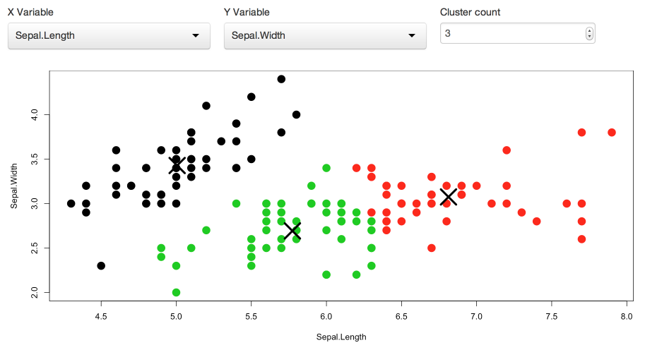
The rmdexamples package includes an example of Shiny widget implemented in this fashion. The kmeans_cluster function takes a single “dataset” argument and returns a Shiny widget. You can use it within an R Markdown document like this:

```{r, echo = FALSE}
library(rmdexamples)
kmeans_cluster(iris)
```

This is what the widget looks like inside a running document:

kmeans_cluster <- function(dataset) { 
  
  require(shiny)  
  
  shinyApp(
    ui = fluidPage(
      fluidRow(style = "padding-bottom: 20px;",
        column(4, selectInput('xcol', 'X Variable', names(dataset))),
        column(4, selectInput('ycol', 'Y Variable', names(dataset),
                              selected=names(dataset)[[2]])),
        column(4, numericInput('clusters', 'Cluster count', 3,
                               min = 1, max = 9))
      ),
      fluidRow(
        plotOutput('kmeans', height = "400px")  
      )
    ),
    
    server = function(input, output, session) {
      
      # Combine the selected variables into a new data frame
      selectedData <- reactive({
        dataset[, c(input$xcol, input$ycol)]
      })
      
      clusters <- reactive({
        kmeans(selectedData(), input$clusters)
      })
      
      output$kmeans <- renderPlot(height = 400, {
        par(mar = c(5.1, 4.1, 0, 1))
        plot(selectedData(),
             col = clusters()$cluster,
             pch = 20, cex = 3)
        points(clusters()$centers, pch = 4, cex = 4, lwd = 4)
      })
    },
    
    options = list(height = 500)
  )
}

Widget Size and Layout

Shiny widgets may be embedded in various places including standard full width pages, smaller columns within pages, and even HTML5 presentations. The following guidelines will help ensure that widget size and layout works well in all of these contexts:

1. Use fluidPage with the responsive = FALSE parameter. This ensures that as the width of a widget gets smaller that elements within it scale smaller as well (and don’t wrap).

2. Ensure that the total height of the widget is no larger than 500 pixels. This isn’t a hard and fast rule, but HTML5 slides can typically only display content <= 500px so if you want your widget to be usable within presentations this is a good guideline to follow.

The example above follows both of these guidelines, specifying a total height of 500px and a height of 400px for the plot (to leave room for the controls above it). Note that height should be specified both on the plotOutput call as well as the renderPlot call.

Another approach would be to add an explicit height parameter to the function which creates the widget (default to 500 so it works well within slides).